RaSQL (Recursive-aggregate-SQL)

RaSQL language is an extension of the current SQL standard by allowing the use of the aggregates such as min, max, count and sum in the Common Table Expression (CTE) by which recursive queries can be expressed in the current standard. The exclusion of aggregates from the Recursive CTE of current standards was largely due to concerns about semantics and implementation caused by the non-monotonic nature of aggregates, since this can compromise the least-fixpoint semantics of these queries. Therefore, the current SQL standard merely supports queries that are stratified w.r.t. aggregates, i.e., the recursive queries (with no aggregates) produce their results first and only after that the aggregates can be applied.

Fortunately, it was recently shown that recursive queries with aggregates that satisfy a Pre-Mappability PreM condition produce the same results as the stratified program; thus they are semantically equivalent but evaluate much more efficiently than their stratified counterparts - and actually they are safe in many situations when the stratified queries are not. Moreover, by using min, max, count and sum in programs that satisfy PreM, we can write queries that express most polynomial-time algorithms of frequent usage.

We use the classical Bill of Materials (BOM) example, an important recursive query application in SQL:99, to illustrate the syntax and semantics of RaSQL and the PreM property. In our simple version of BOM, we have the following two base relations:

assbl(Part, Spart)
basic(Part, Days)

For each item, the assbl relation describes its immediate subparts. Not all items are assembled: basic parts are purchased directly from external suppliers and will be delivered in a certain number of days, which is described in the basic table. Without loss of generality, we assume a part will be ready the very same day when its last subpart arrives. Thus, the number of days required for the an item to be ready is the maximum day when each of its subparts is delivered.

In SQL:99, the BOM query can be expressed as follows:

/*Q1: Days Till Delivery by a Stratified Program*/
WITH recursive waitfor(Part, Days) AS    	
	(SELECT Part, Days FROM basic)
		UNION 
	(SELECT assbl.Part, waitfor.Days
	FROM assbl, waitfor
	WHERE assbl.Spart = waitfor.Part)
SELECT Part, max(Days) FROM waitfor GROUP BY Part

RaSQL still supports this query, but also supports an equivalent and much more efficient version as below.

/*Q2: The Equivalent Endo-Max Program*/
WITH recursive waitfor(Part, max() as Days) AS
   (SELECT Part, Days FROM basic)
      UNION 
   (SELECT assbl.Part, waitfor.Days
    FROM assbl, waitfor
    WHERE assbl.Spart = waitfor.Part)
SELECT Part, Days FROM waitfor

Note that from a syntax point of view, RaSQL query only makes a small change to replace the stratified max (stratified aggregate means it can only be applied to the result of recursive evaluation, not within the recursive evaluation process) used in Q1 by the max aggregate in the recursive CTE head of Q2. However, it is non-trivial to show that Q1 and Q2 are equivalent semantically and evaluate to the same result, which is discussed below.

RaSQL (Recursive-aggregate-SQL)

1. Semantics

The semantics for query Q1 and Q2 are defined by naive fixpoint evaluation shown in Algorithm 1 and 2, where the following abbreviations are used:

wf = waitfor
⋈ = ⋈ (assbl.Spart=wf.Part)
𝜋 = 𝜋 (assbl.Part=wf.Days)
max = Part max Days

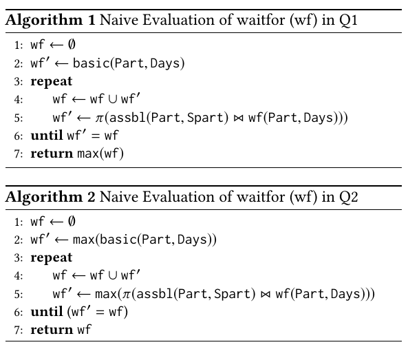
We denote the Relational Algebra (RA) expression used in line 5 of Algorithm 1 as T, which derives the new wf' from the old wf. The operators used by T are union, join and project, which are monotonic and guarantees that when wf'=wf, we obtain the least fixpoint solution of equation wf=T(wf), which defines the formal semantics of the Recursive CTE Q1. The last line in Q1 contains a non-monotonic max aggregate which is applied to wf when the fixpoint wf=T(wf) is reached. This computation is performed at line 7 of Algorithm 1, which computes the perfect-model for query Q1 that is stratified w.r.t. max.

Algorithm 2 shows the naive-fixpoint evaluation for Q2. The max aggregate has been moved from the final statement in Q1 to the head of the Recursive CTE in Q2. Thus the maxaggregate which was in line 7 of Algorithm 1 has now been moved to line 1 and 5 of Algorithm 2 - i.e., lines that specify the initial and iterative computation of wf.

This example illustrates that supporting aggregates in the WITH recursive clause requires only simple extensions at the syntax level, and techniques such as semi-naive fixpoint and magic sets also require simple extensions when aggregates are allowed in recursion. However aggregates in recursion raise major semantics issues caused by their non-monotonic nature. Fortunately the recent introduction of the PreM property has enabled much progress on this problem. In fact, the PreM holds for this example which indicates Q1 and Q2 will produce the same results (concrete semantics) and Q2 has a minimal fixpoint semantics that is equivalent to the perfect model semantics of Q1 (abstract semantics).

2. The PreM property

If T(R1, …, Rk) is a function defined by RA we say that a constraint γ, is PreM to T(R1, …, Rk) when the following property holds:

γ(T(R1, …, Rk)) =  γ(T(γ(R1), …, γ(Rk)))

PreM for union has long been recognized and used as a cornerstone for parallel databases and MapReduce. Moreover the PreM property also holds for join and other operators, which provides a general solution to the semantic problem of having aggregates in recursive queries.

Consider the RA expression T used in line 5 of Algorithm 2, which computes the new value of wf' from its old value wf. The PreM property holds for max if max(T(wf)) = max(T(max(wf))), i.e. if the following relational expressions are equivalent:

max(𝜋 (assbl(Spart,Part) ⋈ wf(Part,Days)))= max(𝜋 (assbl(Spart,Part) ⋈ max(wf(Part,Days))))

This PreM equality states that the max waitfor days for a part is the max of the max of days for each of its subparts. For simple queries such as this, proving the PreM property is straightforward. Moreover, powerful techniques are available for proving that complex expressions of RA and arithmetic operators are PreM w.r.t. extrema and other aggregates.

With the PreM property holding, we can now observe that max(wf(Part,Days)) simply denotes the application of max to the previous step in the computation of Algorithm 1, by applying the join and the PreM rule interchangeably, we can derive Algorithm 2 from Algorithm 1:

max(wfn(Part,Days))
= max(𝜋 (assbl(Spart,Part) ⋈ wfn-1(Part,Days)))
= max(𝜋 (assbl(Spart,Part) ⋈ max(wfn-1(Part,Days)))
= max(𝜋 (assbl(Spart,Part) ⋈
max(𝜋 (assbl(Spart,Part) ⋈ max(wfn-2(Part,Days))))
…
= max(𝜋 (assbl(Spart,Part) ⋈ …
max(𝜋 (assbl(Spart,Part) ⋈ max(basic))))
(Due to limited space, union is omitted, given that PreM holds for union)

Symmetrically, if we start from Algorithm 2, we see that max(wf(Part,Days)), i,e., the max applied to the previous step in the iteration, can be removed without changing the result. Therefore, starting at line 2, and repeating this reasoning for each successive step, we can remove each max from Algorithm 2 - except the one at the last step, that will actually be applied at line 7. In other words, we find that PreM allows us to transform Algorithm 1 into Algorithm 2 and vice-versa, thus providing a robust proof of the equivalence of the operational semantics of Q1 and Q2. We also have that at the pure declarative level, the abstract semantics of Q1 and Q2 coincide, since the minimal fixpoint semantics for Q2 coincides with the perfect model of Q1.

In addition to min and max, the PreM condition entails the use of count and sum in recursion. This is because, the count can be modeled as the max applied on the continuous monotonic count which can be freely used in recursion, and similar property hold for the sum of positive numbers. Thus for our BOM example, we can use a query similar to Q2 to efficiently compute the count of items used in an assembly, or to sum their costs.

RaSQL (Recursive-aggregate-SQL)

Examples

We provide a list of example queries expressible in RaSQL: Example 1-3 are classical graph queries; Example 4-8 demonstrate the power of aggregates in recursion to a broad range of application scenarios.

1. Single-Source-Shortest-Path (SSSP):

/*Base tables:*/
edge(Src: int, Dst: int, Cost: double)

WITH recursive sp (Dst, min() AS Cost) AS
  (SELECT 1, 0)
   UNION
  (SELECT edge.Dst, sp.Cost + edge.Cost FROM sp, edge
   WHERE sp.Dst = edge.Src)
SELECT Dst, Cost FROM sp

The Single-Source-Shortest-Path (sssp) query finds paths with minimal costs from a given source node to all other nodes in the graph. The base relation edge(Src, Dst, Cost) describes all weighted directed edges in the graph. In this example, the sp relation is initialized with the source node 1. The cost to other nodes are iteratively computed by joining the existing weighted paths with the base relation edge, and the min aggregation is used to find the minimal path.

2. Connected-Components (CC):

/*Base tables:*/
edge(Src: int, Dst: int)

WITH recursive cc (Src, min() AS CmpId) AS
  (SELECT Src, Src FROM edge)
   UNION
  (SELECT edge.Dst, cc.CmpId FROM cc, edge
	WHERE cc.Src = edge.Src)
SELECT count(distinct cc.CmpId) FROM cc

The idea of the Connected-Components query is label propagation: In the base case, each node is initially assigned its own id as the CmpId; In the recursive case, each node is receiving CmpId propagated from its neighbors in each iteration. The min aggregation restricts the CmpId of a node to be the minimal id received. The final result is calculated by counting the distinct number of CmpIds as all nodes within a single connected component will have the same (minimal) CmpId when the fixpoint is reached.

3. Count Paths:

/*Base tables:*/
edge(Src: int, Dst: int)

WITH recursive cpaths (Dst, sum() AS Cnt) AS
  (SELECT 1, 1)
   UNION
  (SELECT edge.Dst, cpaths.Cnt FROM cpaths, edge
   WHERE cpaths.Dst = edge.Src)
SELECT Dst, Cnt FROM cpaths

The Count Paths query computes number of paths from a node to all nodes in a graph. Given the start node, the base case initializes the count to itself as 1. In the recursive case, the number of paths from the start node to another node is iteratively computed by adding up the path count from the start node to an intermediate node, which directly connects to the destination code.

4. Delivery (BOM):

/*Base tables:*/
basic(Part: int, Days: int)
assbl(Part: int, Sub: int)

WITH recursive actualdays (Part, max() AS Mdays) AS
  (SELECT basic.Part, basic.Days FROM basic)
   UNION
  (SELECT assbl.Part, actualdays.Mdays
   FROM assbl, actualdays
   WHERE assbl.Sub = actualdays.Part)
SELECT Part, Mdays FROM actualdays

The delivery query computes the number of days until delivery for items in the application of BOM (Bill of materials). An item is either a basic item or needs to be assembled from other items. The basic item is represented by the base relation basic(Part, Days), and the assembling relationship between items is represented by assbl(Part, Sub). The basic item is delivered in pre-given days and the assembled item is delivered as soon as all its sub components are delivered (assuming assembling does not take extra days). In the base case, it computes the delivery days for all basic items. In the recursive case, it derives the delivery days for each item that needs assembling by finding the maximum delivery days among all its sub components.

5. Management:

/*Base tables:*/
report(Emp: int, Mgr: int)

WITH recursive empCount (Mgr, count() AS Cnt) AS
  (SELECT report.Emp, 1 FROM report)
   UNION
  (SELECT report.Mgr, empCount.Cnt
   FROM empCount, report
   WHERE empCount.Mgr = report.Emp)
SELECT Mgr, Cnt FROM empCount

The management query calculates the total number of employees that a manager directly/indirectly manages in a large corporation. The base relation report(Emp, Mgr) describes the relationship between an employee and his/her manager. In the base case, the employee count for everyone is initialized to 1 (him/herself). In the recursive case, the employee count of a manager is iteratively computed by adding up the employee count of his/her direct reporters.

6. MLM Bonus:

/*Base tables:*/
sales(M: int, P: double)
sponsor(M1: int, M2: int)

WITH recursive bonus(M, sum() as B) AS
  (SELECT M, P*0.1 FROM sales)
   UNION
  (SELECT sponsor.M1, bonus.B*0.5 FROM bonus, sponsor
   WHERE bonus.M = sponsor.M2)
SELECT M, B FROM bonus

Some companies adopt a multi-level marketing model to sell products, i.e. salesmen in such a company form a pyramid hierarchy: new members are recruited into the company by old members (sponsors), and get products from their sponsors. To incentive its members to recruit more people to sell more products, the company rewards each member by the bonus. The bonus is not only based on his/her own personal sales, but also the sales of each member in the network that he/she directly/indirectly sponsored. The query calculates the bonus that such a company needs to distribute to its members. The sales relation describes the gross profit P that each member makes, and the sponsor relation denotes the sponsor relationship. In the base case, it calculates the bonus that a member earns through the products that sold by himself/herself . In the recursive case, it calculate the bonus that derived from the sales of each member that he/she directly/indirectly sponsors.

7. Interval Coalesce:

/*Base tables:*/
inter(S: int, E: int)

CREATE VIEW lstart(T) AS
  (SELECT a.S FROM inter a, inter b
   WHERE a.S ≤ b.E
   GROUP BY a.S HAVING a.S = min(b.S))

WITH recursive coal (S, max() AS E) AS
  (SELECT lstart.T, inter.E FROM lstart, inter
   WHERE lstart.T = inter.S)
   UNION
  (SELECT coal.S, inter.E FROM coal, inter
   WHERE coal.S ≤ inter.S AND inter.S ≤ coal.E)
SELECT S, E FROM coal

The Interval Coalesce query finds the smallest set of intervals that cover input intervals. It is one of the most frequently used queries in temporal databases. However, it is notoriously difficult to write correctly in SQL. Here, we express it succinctly using RaSQL with the help of max aggregate. In the first part, a non-recursive view called lstart is created to find all left start points of intervals that are not covered by other intervals (except itself), using self-join of the base relation inter(S, E). In the second part, the recursive view coal(S, E), which represents the final coalesced intervals, is computed by iteratively extending the end points of intervals having the left starting points in lstart through merging other intervals which cover these end points.

8. Party Attendance:

/*Base tables:*/
organizer(OrgName: str)
friend(Pname: str, Fname: str)

WITH recursive attend(Person) AS
  (SELECT OrgName FROM organizer)
   UNION
  (SELECT Name, Ncount FROM cntfriends
   WHERE Ncount >= 3),
recursive cntfriends(Name, count() AS Ncount) AS
  (SELECT friend.FName, friend.Pname
   FROM attend, friend
   WHERE attend.Person=friend.Pname)
SELECT Person FROM attend

More complex queries can be expressed in the mutual recursion fashion - the definition of a recursive relation includes references to other recursive relations. In this example, we want to know people who will attend the party - a person will attend the party if and only if three or more of his/her friends attend, or he/she is the organizer. The attend relation records people who will attend the party. The cntfriends relation records the number of a person's friends who will attend the party. These two relations are mutual recursive to each other and uses the results produced from the other in each recursive iteration.

9. Company Control:

/*Base tables:*/
shares(By: str, Of: str, Percent: int)

WITH recursive cshares(ByCom, OfCom, sum() AS Tot) AS
  (SELECT By, Of, Percent FROM cshares)
   UNION
  (SELECT control.Com1, cshares.OfCom, cshares.Tot
   FROM control, cshares.ByCom
   WHERE control.Com2 = cshares.ByCom),
recursive control(Com1, Com2) AS
  (SELECT ByCom, OfCom, Percent
   FROM cshares
   WHERE Percent > 50)
SELECT ByCom, OfCom, Tot FROM cshares

The Company Control query was proposed by Mumick, Pirahesh and Ramakrishnan to calculate the complex controlling relationships between companies. Companies can purchase shares of other companies. In addition to the shares that a company owns directly, a company A owns shares that are controlled by a company B when A has a majority (over 50% of the total number) of B's shares. A tuple (A, B, 51) in the base relation shares indicates company A directly owns 51% of the shares of company B. This query also uses the mutual recursion: the cshares view recursively computes the percentage of shares that one company owns of another company while the control view decides whether one company controls another company.

RaSQL Publications

• Jiaqi Gu, Yugo H. Watanabe, William A. Mazza, Alexander Shkapsky, Mohan Yang, Ling Ding, Carlo Zaniolo. RaSQL: Greater Power and Performance for Big Data Analytics with Recursive-aggregate-SQL on Spark, SIGMOD 19. ACM DL

• Carlo Zaniolo, Mohan Yang, Matteo Interlandi, Ariyam Das, Alexander Shkapsky, Tyson Condie. Declarative BigData Algorithms via Aggregates and Relational Database Dependencies, AMW 18.

• Carlo Zaniolo, Mohan Yang, Ariyam Das, Alexander Shkapsky, Tyson Condie, Matteo Interlandi. Fixpoint semantics and optimization of recursive Datalog programs with aggregates, TPLP 17. arXiv